

Since launch, Flashduty has stored alerts, alert events, incidents, and incident timelines in MongoDB. This year we moved that storage to PostgreSQL. We switched 22 data families one at a time, with no maintenance window.
We're writing this because we couldn't find a detailed production runbook for this kind of migration when we started. What follows is our workload, our constraints, and what we did. Take it as a reference, not a recipe.
The short version: the problem was how the data was physically organized, and the choice of engine came second. Our hot data sits in a few tenants and in recent weeks. MongoDB made all of it share one set of indexes, one disk, and one cache. PostgreSQL partitioning lets us store data the way we read it.
The post answers four questions in order: why we migrated, how the new storage is designed, how we moved over without downtime, and what the results and problems were. It ends with what we learned about choosing a database.
Why we migrated
We migrated because the business grew. With more and more customers, the original storage design could no longer keep up.
MongoDB itself wasn't the problem. It served us well for four years. Alert labels are arbitrary key-value pairs, so a document model with no upfront schema let the product move fast early on. Nodes in our core cluster ran for more than a year without a restart.
WiredTiger's block compression is good too: data on disk is about a quarter of its logical size. After the migration we measured PostgreSQL's uncompressed heap at roughly MongoDB's logical size, so the same data takes more disk on PostgreSQL.
The problems came down to the three below. The fourth subsection explains why a MongoDB sharded cluster doesn't fix them.
Hot spots and uneven data
Data volume differs by more than a thousand times between tenants. Some customers send more than 1 million alerts a day. Most send fewer than 1,000.
Our first design was simple sharding in the application: hash the tenant ID and pin each tenant to one table. A hash decides which table a tenant lands in, not how big that table gets, so the few tables holding large tenants grew far larger than the rest.
On-premises deployments usually have a single tenant, so all their data sat in one table and the sharding did nothing.
No hot/cold tiering
Access hits the last month, but most of the data is old:
- The console queries the last 30 days by default, and we estimate about 99% of queries fall in that range. During one weekday peak, fewer than 0.5% of reads touched data older than 90 days.
- In another sample, data older than nine weeks received no writes in an hour.
- We keep incident data for about a year. By age, data older than 90 days is about two-thirds of the total.
In MongoDB this data wasn't separated by time, so every query pattern needed an index covering all history. Indexes added up to about 94% of the compressed data size and about 25 times the WiredTiger cache limit. The cache was always full and pages kept swapping in and out.
We used $indexStats to check more than a year of index access: indexes that were never used made up less than one hundred-thousandth of the total. There was nothing to drop.
Too many slow queries
The first two problems made things slow. With a 100 ms slow-log threshold, we logged more than 10,000 entries a day.
Writing one alert updated eight index trees. Expiry could only delete documents one at a time, and each delete updated every index, so the nightly cleanup was a top source of slow-log entries.
The clearest case is counting. Alert and incident lists show a total, and MongoDB doesn't keep filtered counts:
- An unfiltered count reads collection metadata.
countDocumentswith a filter runs an aggregation that counts matching records one by one.- It can count index keys alone (COUNT_SCAN) only when every filter condition falls in one contiguous range of a single index.
Our lists filter on any mix of status, severity, channel, labels, and time. Most combinations narrow the range with an index and then fetch each document to check the rest. More data means a bigger candidate range, and most of those old documents aren't cached, so they come from disk.
We capped counts at 1,000, but a cap only helps when matches are dense. With a strict filter and few matches, the query scans the whole candidate range and never reaches 1,000.
Two things followed:
- One group of slow-log entries stopped at almost exactly 2 seconds: these counts hitting the client timeout. The list opened, but the total never arrived.
- A count of active incidents over 30 days grouped by severity took 19.5 seconds at its slowest.
More memory only delayed the problem. Doubling the cache would cover about a year of growth and raise the annual cost to about 1.5 times.
A sharded cluster doesn't fix these
Sharding and partitioning solve different problems, and what we lacked was partitioning. After four years on MongoDB, a sharded cluster was the obvious next step, so we evaluated it carefully first.
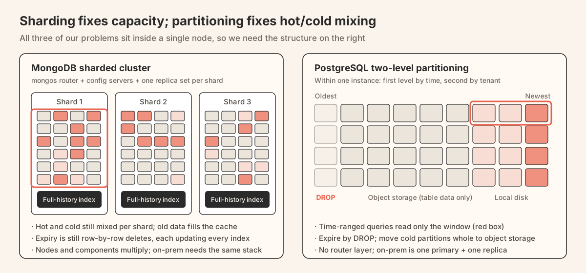
Sharding decides which machine holds a record. It solves "one machine can't store or serve this". Partitioning splits a table along the way you access it, so you can drop, move to another storage tier, or maintain each piece on its own.
MongoDB can shard, but it has no table partitioning. After sharding, each shard still holds collections and indexes that mix all of history. All three problems above lived inside a single node, and no shard key changes that:
| Shard key | Write distribution | Hot/cold data and cleanup |
|---|---|---|
| Account + time | A large tenant splits into several chunks, but its writes always land in the chunk holding the newest time range | Each shard mixes hot and cold data, and expiry still deletes one document at a time |
| Time | All writes go to the newest shard | Old chunks can move away, but the balancer migrates them one chunk at a time |
| Hashed | Writes spread evenly | A list query by time range hits every shard, and hot and cold data are fully scattered |
We also went through the workarounds MongoDB offers:
- TTL indexes delete expired data automatically, but still one document at a time in the background, and each delete updates every index. That's the same cost as our nightly cleanup.
- Zone sharding can pin chunks with old data to cheaper shards. The balancer still moves data chunk by chunk, and each shard's indexes still cover everything it holds.
- Time series collections target measurements that aren't modified after they're written. On 5.0, the version we ran, they don't support updates. Newer versions allow updates, but data is still stored in buckets, which doesn't fit business records that change often, like counters, status changes, and assignees.
- Online Archive moves old data to object storage automatically, but only on MongoDB Atlas. Our SaaS ran on a regional cloud provider's managed service, and on-premises deployments can't use it either.
- Creating a collection per month in the application means building your own partitioning. On top of the existing hash sharding, the collection count would grow 12 times. Indexes would be created by script, and code would decide which collections to query. While investigating, we found that one set of indexes existed on only about a third of our tables. The rest still had the old structure, and nobody had noticed.
So MongoDB can do it, but only if we build partitioning ourselves in the application and maintain it forever.
Cost and operations don't favor it either. Each shard in a sharded cluster is its own replica set, plus config servers and mongos routers, so the node count multiplies. On-premises deployments would need the same full set of components.
Since partitioning was what we lacked, the next step was a database with native partitioning and a storage design built around it.
The new storage design
The new design does one thing: it stores data the way we read it. Heavy tenants get their own space, and hot and cold data are separated by time.
We chose PostgreSQL. Partial indexes, multi-level partitioning, GIN indexes over arbitrary label keys, array operations, and advisory locks are all built into PostgreSQL. On MySQL they'd need extra tables or application logic.
The subsections below cover four things in turn: how tables are partitioned, how queries touch only the relevant partitions, how cold data moves away, and how the two environments are deployed. The last one follows a single alert through all of them.
Two-level partitioning: time first, tenant second
The alert, alert event, incident, and timeline tables share one two-level structure. Time decides hot and cold; account isolates the heavy tenants.
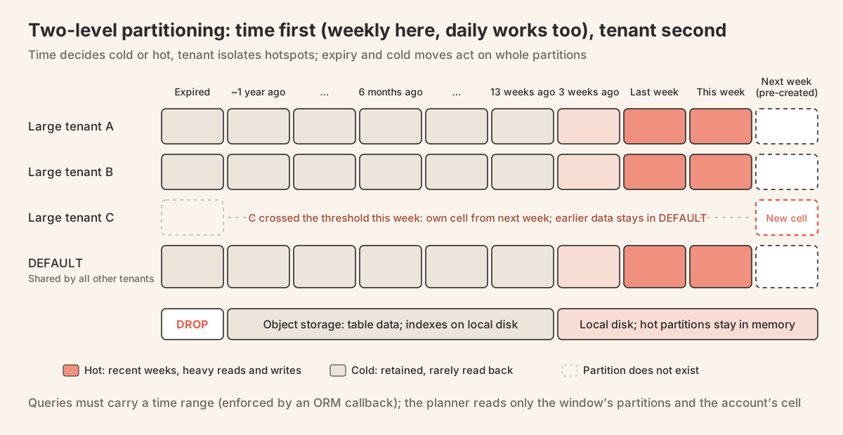
The first level is RANGE by time. Inside each time partition, the second level is LIST by account: each large tenant gets its own partition and the rest share a DEFAULT partition.
Partition size decides the time granularity. The figure uses weeks, and you can go to days with more data.
Promoting a large tenant moves no history. We can't know in advance which account will become large. A nightly job counts rows per account in the DEFAULT partitions, and an account over the threshold gets its own partition starting with the next time partition.
That partition is still empty, so adding a LIST partition is a metadata change that finishes instantly. History stays in the old DEFAULT partition and is dropped with its time partition when it expires.
That's why time is the first level. With account as the first level, promotion would mean three steps: DETACH the DEFAULT partition, move the data, and ATTACH it back. While rows moved, other tenants' data would vanish from the parent table. During validation we tried both orders, and pruning selected exactly the same partitions.
Queries touch only the relevant partitions
Partitioning only helps when a query is pruned to a few partitions, so pruning can't rest on convention. Code has to enforce it.
Queries without a time range are rejected. With a time range in the query, PostgreSQL only touches the relevant partitions during planning and execution. But one query without a time range scans every partition.
So we added a check in an ORM callback: any statement on a partitioned table without a time range is rejected. After rollout, statements that scanned the full retention dropped from 183 per 10 minutes to zero.
Lookups by ID must prune too. In MongoDB, alert and incident IDs are ObjectIds, whose first 4 bytes are a creation timestamp in seconds. Our API also supports lookups by ID.
The IDs didn't change in PostgreSQL, but a query with only an ID and no time range would be rejected by the check above. So we read the time out of the ID and turn it into the query's time range:
- We generate IDs for new data ourselves, the same way as ObjectId, except the first 4 bytes hold the partition key's time. ID time equals the partition key, so a lookup checks one hour on either side and usually lands in one or two partitions.
- For old data, ID time is the write time, while the partition key is the business time, such as when the alert started. We checked every historical partition: the two differ by at most 29 days. So an old ID's lookup range extends 30 days before its ID time, about five or six partitions. Once old data ages out of retention, the wide window goes away.
Partial indexes shrink the hot path. MongoDB supports partial indexes too, and they weren't why we switched engines, but combined with partitioning they make a clear difference. Deduplication asks whether an alert still has an active record, and active alerts are a small fraction, so we built a separate partial index for them.
During validation, for one large tenant, this index was about a tenth the size of the full index. Loading the active alerts page went from 308 ms to 0.4 ms, and pages read went from 132,000 to 59. Writing one alert now updates three or four index trees instead of eight.
Transactions and advisory locks guard concurrent writes. Alert merges and the cascading writes between incidents and alerts run in a single transaction. Deduplication takes pg_advisory_xact_lock on the alert key, a second concurrency guard on top of Kafka's per-key partitioning.
What this did for counts. A PostgreSQL count also counts rows one by one; there's no shortcut. The difference is that after pruning it only counts the few partitions in the time window that hold that tenant, so the range no longer grows with history.
During validation we took the 18 slowest query types from the production slow log and reran them on PostgreSQL:
- The capped count that couldn't finish in 2 seconds on MongoDB took 23 ms.
- The grouped count by severity went from 19.5 seconds to 250 ms.
The validation instance was smaller, had no concurrency, and held only 90 days of data, so read these numbers as orders of magnitude, not exact ratios.
Moving cold data to object storage
With partitions, the data lifecycle is managed a whole partition at a time. A scheduled job creates future partitions ahead of time, old partitions move to object storage, and expired partitions are dropped. A drop is a metadata operation with no row-by-row deletes.
Of the three, only moving cold data went badly. It took more time than any other part of the migration, and we changed the design four times.
The goal was simple. For partitions older than about three months, move only the table data to object storage and keep indexes on local disk. Reads fetch pages from object storage on demand. Object storage costs about one-fifteenth as much as cloud disk. The trade-off is slower cold reads: a lookup by ID on cold data has a p50 of 4.8 ms, against 2.3 ms for the same query on cloud disk.
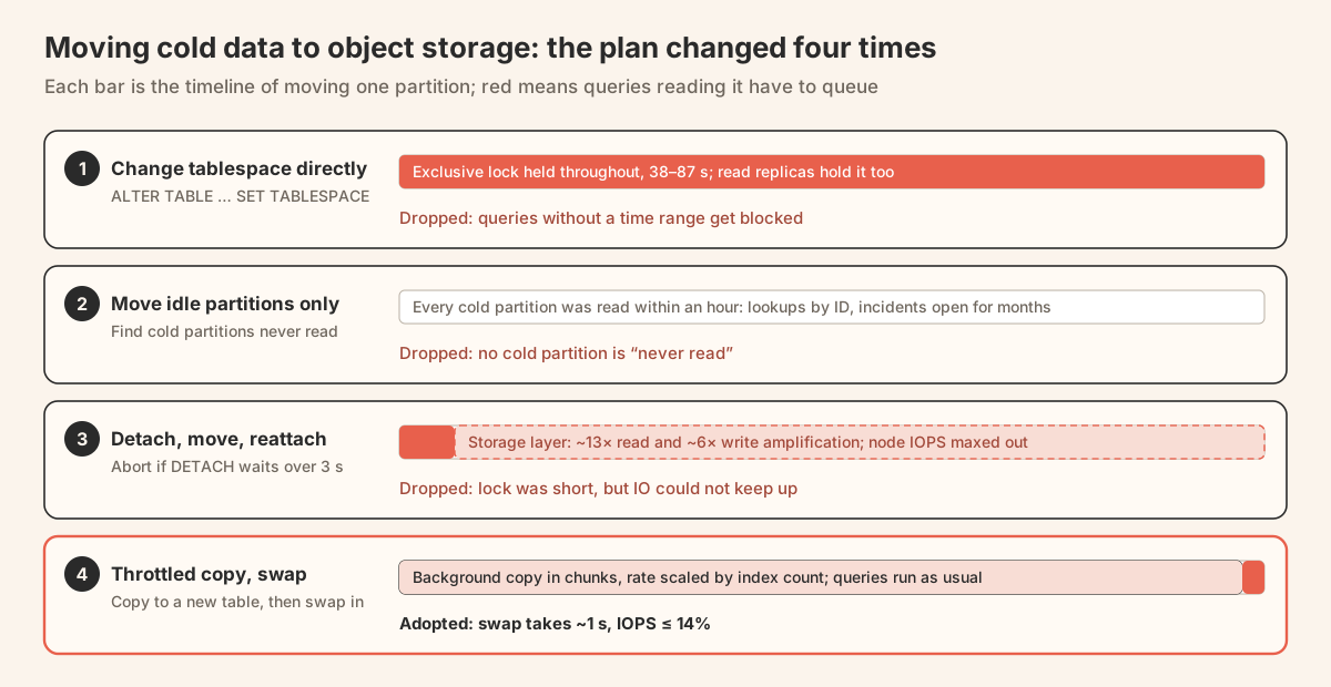
First: change the tablespace in place. ALTER TABLE ... SET TABLESPACE holds an exclusive lock the whole time. Moving one partition took 38–87 seconds, and read replicas held the same lock.
A query without a time range touches every partition, so it waited behind the one being moved. This is when the rule in the previous subsection, rejecting queries without a time range, was set.
Second: move only partitions nobody reads. We counted access to each cold partition over an hour, and every one had been read.
Some reads were lookups by ID. Others came from incidents left open for months: counting their alerts reads from the incident's start time through today. No cold partition goes unread, so this idea was dead.
Third: detach, move, reattach. We first added a CHECK constraint matching the partition bounds, so ATTACH wouldn't need a validation scan. Then DETACH (giving up if the lock wait passed 3 seconds), change the tablespace, and ATTACH.
That solved the lock. But moving 15 GB caused about 13 times the reads and 6 times the writes at the storage layer and hit the node's IOPS cap within minutes, so we stopped.
Fourth: copy at a controlled rate and swap in under a short lock. This is the design we run today:
- Create a new table on the object storage tablespace and copy data in 4,096-page chunks, running VACUUM FREEZE after each chunk.
- Scale the copy rate down with the number of indexes, since each index adds another write. The job runs in a fixed nightly window with a time budget.
- After the copy, check whether the source partition got new writes during the copy, and swap the copy in under a short lock only if it didn't. A copy that doesn't get swapped in is cleaned up on the next run.
It now moves two partitions a night. ATTACH takes about 1 second, primary IOPS stays under 14%, and there's no lock wait.
We hit two more problems here.
A bug in the managed service's kernel. When a read replica read cold data, the reference it left on the primary's cache was never released, and later drops or VACUUM truncation of cold partitions hung. We paused cold moves and expiry until the vendor fixed the kernel and we verified the fix with a synthetic reproduction.
Transaction ID freezing. The last block or two of each copied table, and old partitions no longer written after backfill, were never frozen, and autovacuum wouldn't visit them again. Their transaction ID ages would hit the limit together and trigger forced anti-wraparound VACUUMs at the same time, scanning hundreds of GB.
We ran VACUUM (FREEZE) table by table during off-peak hours ahead of time to bring the ages down.
Deployment: SaaS and on-premises
The same design has to run in two environments with very different operations, so we planned deployment for each.
SaaS uses a cloud provider's managed service. As long as it speaks the PostgreSQL protocol, we prefer offerings with a proxy layer:
- The application connects only to the proxy, which handles primary failover faster.
- Data stays hot-standby across availability zones, so one zone failing doesn't take the whole service down.
- Cold data moves to S3-compatible object storage.
The managed service provides these features; our code uses only the standard PostgreSQL protocol.
On-premises stays simple. On-premises customers run their own databases, and we only require a common setup such as one primary with one replica, or two primaries. Two-level partitioning happens entirely inside one PostgreSQL instance, and the planner prunes to the right partitions, so there's no routing layer or proxy.
Our other Go services already supported PostgreSQL in the on-premises package. MongoDB was the only component without an alternative, so the migration leaves fewer database types to run.
Putting it together: the life of one alert
Follow one row through the pieces above and you get its whole life, from write to drop.
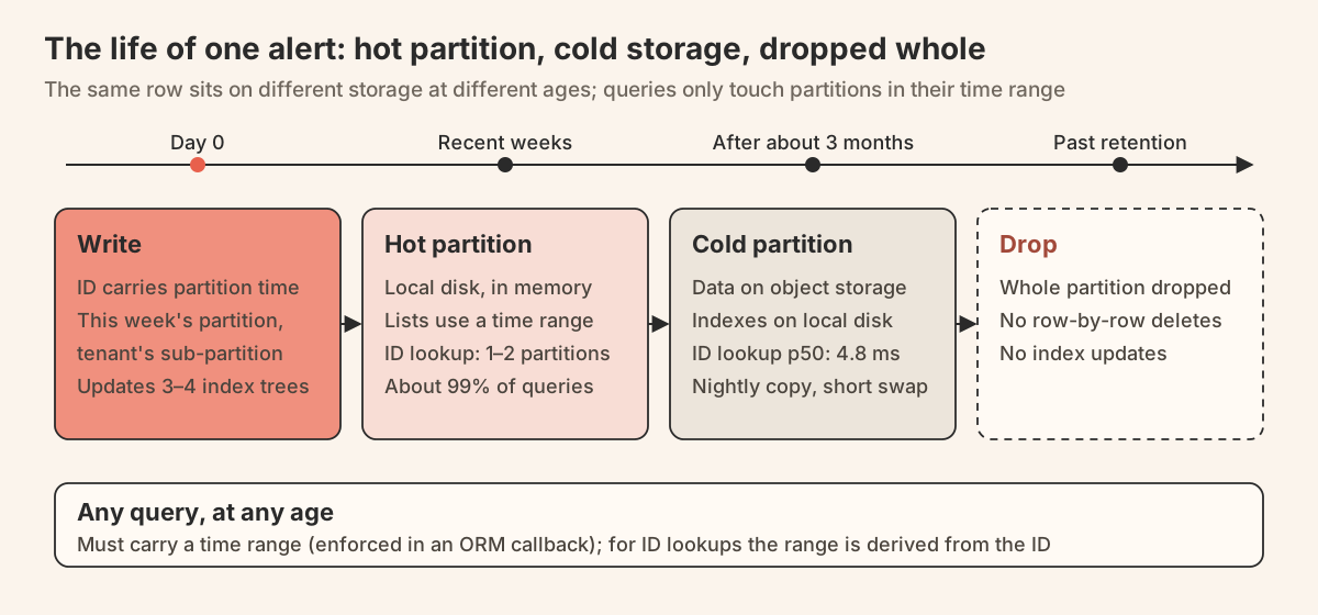
Write. The application generates the ID, with the partition key's time in the first 4 bytes. The row lands in the tenant's sub-partition of this week's partition and updates three or four index trees.
Recent weeks. The partition sits on local disk and stays in memory. List queries carry a time range and touch only the latest few partitions. A lookup by ID reads the time from the ID and lands in one or two partitions.
After about three months. A nightly job copies the partition's table data to object storage and swaps it in. Indexes stay on local disk. The occasional read is slower but still works.
Past retention. The whole time partition is dropped, with no row-by-row deletes and no index updates.
That settles the design. What's left is how to move the data and the traffic over while production keeps writing and reading.
How we migrated
Two constraints shaped the migration: no downtime, and every step reversible within minutes. Everything below follows from those two.
In the model layer, each data family has a Store interface with a MongoDB and a PostgreSQL implementation. The 22 families moved independently. Each had two sets of switches in Redis:
- One for the write mode: MongoDB only, dual write, or PostgreSQL only.
- One for which accounts read from PostgreSQL.
Service processes cache the switches locally for one minute, so a rollback is one key change that takes effect within a minute.
Six stages
Every data family went through the same six stages, and each stage's result is the next one's precondition.
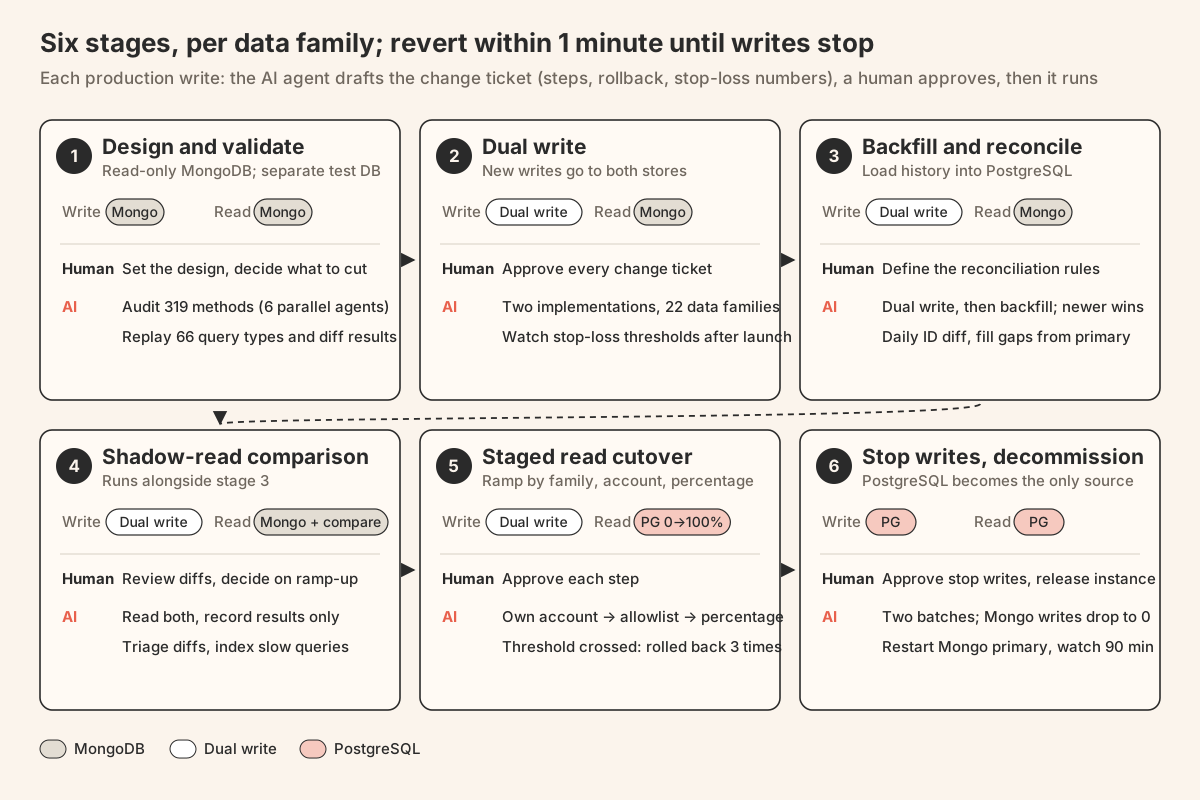
1. Design and validation. First we confirmed the migration was feasible. We listed every model method that touches MongoDB, 319 in total, and confirmed none needed anything a relational database can't do. About 68 had no callers left and could be deleted.
Then we sampled production data by account into a small PostgreSQL instance, replayed 66 query shapes, and compared each query's results on both databases row by row.
2. Dual write. New writes go to both databases. The request returns as soon as the primary store write succeeds. The write to the other database, the shadow store, goes into an in-process queue. If it doesn't succeed within 30 seconds, the account and ID go into a retry set.
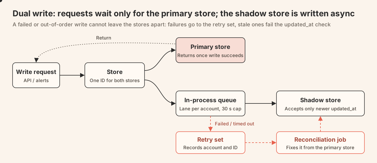
Queues in different processes aren't ordered relative to each other, so every shadow update checks updated_at and only accepts a version newer than the stored row. The application generates IDs before writing, so both sides match.
3. Backfill and reconciliation. Dual write only covers new data, so history has to be backfilled. Backfill uses ON CONFLICT ... DO UPDATE ... WHERE excluded.updated_at >= updated_at, so an old version never overwrites a newer one written during dual write.
Reconciliation compares ID sets on both sides day by day and samples fields. It repairs differences from the account's current primary store. Extra rows on the other side are reported, never deleted.
4. Shadow-read comparison. With the data complete, we still had to confirm queries return the same results. Reads go to both databases. Results are compared and logged, never returned to users. When results differ, we reread after 1 second and after 5 seconds. Differences caused by dual-write lag disappear on reread, and only what's left needs a root cause.
5. Staged read cutover. Only after results matched did real read traffic move. Reads move by data family, account, and percentage. The next subsection covers how.
6. Stop writes and decommission. Once all reads had moved, we stopped MongoDB writes. We switched to PostgreSQL-only writes in two batches: 18 configuration families first, then four time-series families about 20 minutes later. MongoDB writes dropped to zero and the retry sets emptied.
We then turned off the MongoDB alerts, restarted the MongoDB primary, and watched for 90 minutes. No related errors appeared, so we backed up the data to object storage and decommissioned the instances.
Staged read cutover
Read cutover is the only step where users see the new database directly, so the switch has three dimensions that keep the blast radius as small as possible.
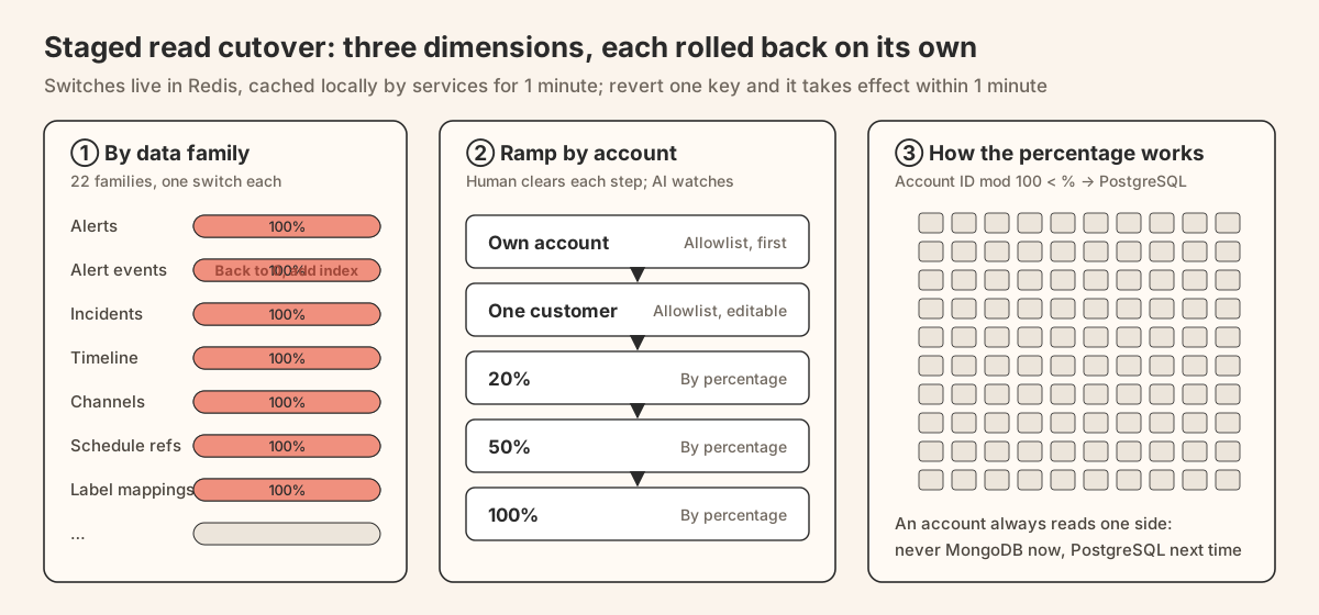
By data family. Each of the 22 families has its own switch. For example, after alert events reached 100%, we found a channel-filtered query missing an index. We set only alert events back to zero, kept the other 21 families at 100%, added the index, and ramped again.
By account allowlist. Accounts on the allowlist read from PostgreSQL. Our own accounts went first, then single customers who agreed to help. You can add or remove one account at a time, so a problem affects only that account.
By percentage. Account ID modulo 100 is compared with the rate, and accounts below it read from PostgreSQL. An account's requests always land on the same side, so it never reads MongoDB on one request and PostgreSQL on the next. We ramped through 20%, 50%, and 100% and rolled back three times along the way; "Four problems we hit" covers why.
Shadow-read comparison uses the same switches, so you can turn it on for allowlisted accounts or a percentage.
Who did what: people and AI agents
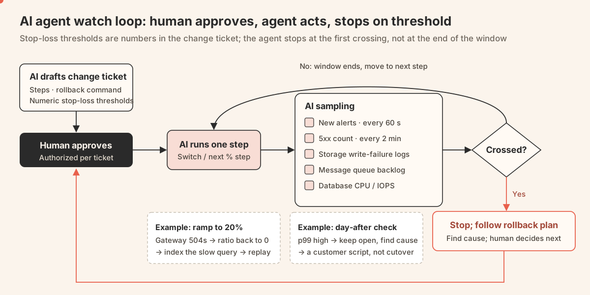
These steps add up to a lot of work, and AI agents did most of it. Humans set the plan, approved every production write, and decided what to do next whenever an agent reported something unusual.
Before the cutover, getting the team fluent in PostgreSQL. The team had mostly worked with MongoDB, so we used AI to build a PostgreSQL tutorial based entirely on our own schema. Its 14 sections cover:
- Connecting, and psql meta-commands.
- Type casts and time columns, binary IDs, and NULL versus JSON null.
- How the 35 tables relate, partitioning rules, retention, and creating tables and indexes.
- 12 typical queries, each next to its old MongoDB version.
By the time anyone had to debug, they already knew how to query the new database.
In design, agents read code and ran validation. The method list from stage 1 came from six agents auditing the whole repository in parallel, with a file and line number for every entry. The agents also set up the environment, wrote the scripts, and ran the query replay and the result comparison.
An earlier belief that "56 GB of indexes can be dropped" was disproved by an agent using more than a year of index access statistics.
In coding, agents wrote both implementations. Two Store implementations per data family, plus tools for dual write, backfill, reconciliation, partition maintenance, and cold moves add up to a lot of code with a very consistent pattern, which suits batch work by agents. Humans reviewed the interface design and the critical concurrency semantics.
In execution, agents drove the rollout and kept watch. For every production write, an agent first wrote a change ticket with the steps, the rollback commands, and stop-loss thresholds in concrete numbers. A human approved it, then the agent ran it.
While running, the agent checked for new alerts every 60 seconds. Every 2 minutes it sampled the stop-loss metrics: 5xx count, storage write-failure logs, message queue backlog, and database CPU and IOPS. Any threshold crossed meant stop.
Two examples from the watch:
- When reads ramped to 20%, the agent saw the gateway start returning 504s. It set the rate back to zero and found the missing indexes from the slow query shapes. The first of the "Four problems we hit" has the details.
- The day after writes stopped, the agent noticed API p99 was higher than the day before. Instead of closing the ticket, it tracked down the cause: a customer's script had started calling one API at high frequency, unrelated to the cutover.
To learn more about Flashduty's AI SRE, see the AI SRE product page.
Results and problems
After the migration we compared production metrics before and after, and wrote down four problems we hadn't expected.
Results
Slow requests on the incident list and incident detail dropped clearly, hot storage shrank by about 40%, and the alert lists' long tail didn't improve.
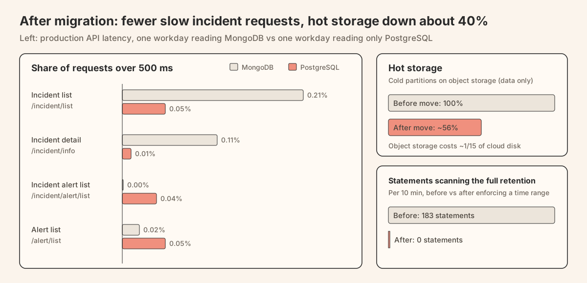
API latency comes from production monitoring. We compared a weekday when everything read MongoDB with a weekday after everything read PostgreSQL. The two days' metrics were collected from different scopes, so we compare only the share of requests in each latency bucket, not request counts.
| Metric | Before (MongoDB) | After (PostgreSQL) |
|---|---|---|
| Incident list: requests over 500 ms | 0.21% | 0.05% |
| Incident list: requests over 1 second | 0.06% | under 0.01% |
| Incident list: p95 | 100–200 ms | under 100 ms |
| Incident detail: requests over 1 second | 0.11% | under 0.01% |
| Both alert lists: requests over 500 ms | 0–0.02% | 0.04–0.05% |
| Hot storage | 100% | about 56% |
| Statements scanning the full retention | 183 per 10 minutes | 0 |
The monitoring histogram has buckets at 10, 100, 200, 500, and 1,000 ms, so p95 only shows which bucket it falls in. The other APIs in the figure had p95 under 100 ms both before and after.
We're still going through the alert lists' slow requests one by one.
Four problems we hit
All four showed up during ramp-up and switching. Each time we stopped it by turning the switch back, fixed the cause, and ramped again.
The shadow path hid slow queries. Shadow reads time out after 1 second, so a query slowed by a missing index on PostgreSQL only showed up as a "shadow read error" and never affected users.
At 20%, three query types started timing out and the gateway returned 504s: regex title search, capped counts, and multi-channel filters. The lesson: before ramping, add indexes for the slow queries on the shadow path. Overall p99 won't show that kind of long tail.
Query plans degraded with many channels. One account followed 276 channels at once, above the limit of 256 for walking the index channel by channel. The query fell back to channel_id = ANY(...), read cold data, and took 4.5–5.6 seconds. We raised the limit to 1,024 and ramped again.
Old and new modes ran side by side during the switch window. Switches have a one-minute local cache, so for a minute after a switch, some processes ran the new mode and some the old.
One data family updated by deleting by ID and recreating. Processes in the two modes generated different IDs, and PostgreSQL hit unique constraint conflicts. We changed that family to delete by business key, fixed it, and switched again.
A global plan cache slowed queries down. Our managed PostgreSQL has a plan cache shared across connections. Once a statement's generic plan was cached, new connections running the same SQL reused it, and one large tenant's query went from 66 ms to 14.8 seconds.
Setting plan_cache_mode = force_custom_plan on the application's database role brought it back to normal.
What we learned about choosing
Looking back, the decisions that mattered were made while choosing, and they aren't specific to MongoDB and PostgreSQL.
Look at the data before the engine. Before choosing, measure three things: how data is distributed across tenants, how access is distributed over time, and how long data is kept and whether it changes after it's written. Our answers were a thousandfold gap between tenants, about 99% of queries within 30 days, and a year of retention with frequent updates. Those three answers are what showed we lacked partitioning, not sharding. Starting from "which database is better" doesn't get you there.
Count operations cost for every deployment environment. SaaS has a managed service behind it; on-premises customers run the database themselves. The same design that means a few more nodes in SaaS means several more components a customer has to learn on-premises. Our on-premises requirement ended up as one primary and one replica, with fewer database types in the package than before.
Usage cost depends on where data sits, not on the engine's price. Switching engines didn't save money on its own, and the same data takes more disk on PostgreSQL. The savings come from two places: expired data is dropped by partition, and cold data moves to object storage at about one-fifteenth the price of cloud disk. Adding memory instead would have raised the annual cost to 1.5 times and bought about a year.
AI lowers migration cost, so you can choose the end state directly. The old reason not to switch databases was the workload: hundreds of methods to rewrite, two implementations side by side, tools for replay, reconciliation, and backfill, and a person watching every step. This time AI agents did most of that.
Once migration is cheaper, stopgaps stop paying off. A collection per month in the application looked like the smallest change at the time. But it needs maintaining forever, the problem stays, and you migrate again later anyway. We went straight to the structure we wanted to end up with.
Go to the end state in one design, but roll it out in steps. Choosing the end state doesn't mean switching in one move. Per-family switches, three cutover dimensions, and one-minute rollback exist so the final design can ship one small step at a time.
Write the costs down up front, and put them where access is rare. No design is free. Our cost is slower reads on cold data, and fewer than 0.5% of reads touch data older than 90 days. The alert lists' long tail is a problem we haven't solved yet.
Enforce rules in code, not by convention. Conventions get bypassed sooner or later: one set of indexes existed on only about a third of the old tables, and nobody had noticed. In the new design an ORM callback checks that every query carries a time range, and a new query that doesn't won't run.
If your data also sits mostly in a few tenants and splits cleanly into hot and cold by time, we hope this record saves you some trial and error.